운영관리

운영관리

Variability and Its Impact on Process Performance

-Waiting Time Problems

개요

• 이번 단원에선 수요가 비정기적으로 도착하는 것이 퍼포먼스에 미치는 영향을 살펴본다.
• 이런 수요의 변동성은 프로세스가 충분한 capacity를 갖고 있다고 해도 고객이 서비스를 받기 위해 대기해야 하는 상황을 만들 수 있다.
• 이 단원에 나오는 프로세스는 Demand < Capacity를 전제로 하기 때문에 Flow rate = Demand로 보아도 무방하다. (원래는 Flow rate = $\min{Demand,\ Capacity}$)
• server가 하나일 경우, 복수일 경우에 대해 살펴볼 것이다.

Variability에 대한 변수

• 기본적으로 Demand, Capacity, Process time, average Inter-arrival time, Average processing time 외에도 다음 변수들을 고려해야 한다.
  • Inter-arrival variation
  • variation of processing time

Notaton and Basic relations (single server)

• Notation
  • $T$ = Flow Time
  • $T_q$ = Time in queue
  • $p$ = average processing time = Activity time = Service time
  • $a$ = average inter-arrival time
  • $R$ = Flow Rate
  • $I_q$ = Inventory waiting
  • $CV_a = \frac{\mathrm{Standard\ deviation\ of\ interarrival\ time}}{\mathrm{Average\ interarrival\ time}}$ = Coefficient of Inter arrival time Variation이 포아송분포를 따른다고 할 때 $CV_a = 1$
  • $CV_p = \frac{\mathrm{Standard\ deviation\ of\ activity\ time}}{\mathrm{Average\ activity\ time}}$ = Coefficient of Inter activity time Variation이 포아송분포를 따른다고 할 때 $CV_p = 1$

• Relations

  Little’s Law

  • $I = R\times T$

  variation과 독립

  • Capacity = $1 / p$
  • Flow Rate = $\min{\mathrm{Demand, Capacity}} = \mathrm{Demand} = 1/a$
  • Utilization = Flow rate / Capacity = $p/a$

  variation에 종속

  • Flow Time = Time in queue + Service Time $T=T_q+p$
  • Inventory = Inventory in process + Inventory in queue $I = I_q\ +\ I_p$
  • Inventory in queue = Flow Rate * Time in queue $I_q=R*T_q$
  • Inventory in process = Flow Rate * service time $I_p\ =\ R*p\ =\ (1/a)p$

additional Notation and relations (multi-server)

• $m$ = number of servers
• Capacity = $m \times 1/ p$
• Utilization = Flow rate / Capacity = $(1/a)/(m\times1/p)\ \ =\ p/(a\times m)$

Single Server Time in queue

• $\mathrm{Time\ in\ queue = Activity\ Time\ *\ \left({\frac{utilization}{1-utilization}}\right)}\ *\ \left({\frac{CV_a^2\ +\ CV_p^2}{2}}\right)$

Multi-server Time in queue

• $\mathrm{Time\ in\ queue = \left({\frac{Activity\ Time}{m}}\right)\ *\ \left({\frac{utilization^{(\sqrt{2(m+1)}\ \ \ )-1}}{1-utilization}}\right)}\ *\ \left({\frac{CV_a^2\ +\ CV_p^2}{2}}\right)$

Pooling in multiple server condition

• 서버가 여러 개일 때 이들 각각에 queue를 배치하는 것 보다 단일 서버들을 묶어서 하나의 큐로부터 수요를 분배받는게 더 효율적이다. (queue를 공유하자)
• n개의 서버 각각에 queue가 있다면
  • a = A * n, p = P, m = 1
• n개의 서버가 하나의 queue를 공유한다면
  • a = A, p = P, m = n

Variability and Its Impact on Process Performance

-Throughput Losses

개요

• 이번 단원은 이전 단원의 연장이다.
• 한가지 조건이 바뀌었는데 customer의 인내가 0으로 수렴하여 대기열이 있을 경우 서비스 받기를 거부한다.
  • 따라서 Inventory queue는 0이 된다.
  • 이전 단원의 전제조건이었던 Capacity > Demand 가 유지된다.
• 이 단원의 중점 사항은 얼마나 많은 수요 Loss가 있을지 예측하는 것이다.
  • 이는 Utilization이 1을 넘을 확률을 알면 구할 수 있다.

Notations and basic relations

• Notations
  • $m$ : number of server
  • $p$ : process time
  • $a$ : inter-arrival time
  • $P_m(r)$ : probability {All $m$ servers ar busy}
• relations
  • $r = \frac{p}{a}$

Flow units lost

= Demand rate * probability that all servers are busy

• $\mathrm{Flow\ units\ Lost = \ }\frac{1}{a} \times P_m(r)$ $(\ \ r = \frac pa\ \ )$

• Flow rate = Demand rate * Probability that not all servers are busy

  $\mathrm{Flow\ rate}\ =\ \frac{1}{a} \times (1-P_m(r))$

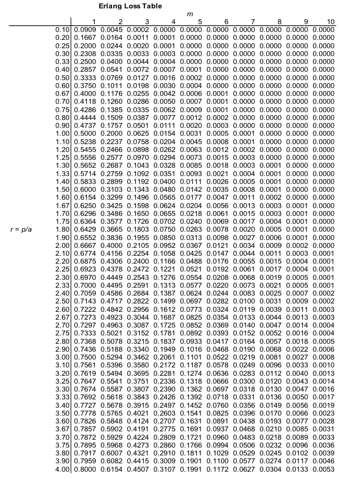
Erlang Loss Table

• Table

  

• Formula

  $P_m(r)=\frac{\frac{r^m}{m!}}{1+\frac{r^1}{1!}+\frac{r^2}{2!}+…+\frac{r^m}{m!}}$

Quality Management, Stastical Process Control (SPC)

개요

• 프로세스의 생산품의 품질이 정확히 동일하기는 매우 어렵다.
  • 기준이 되는 목표 주위로 허용되는 오차가 주워지고, 각 생산품들이 기준에서 얼마나 떨어져 있는지에 대한 수치를 variation이라고 부른다.
• Two types of Variation
  • natural variation
  • abnormally large variation
• 생산물의 variation은 경향성이 있어서 랜덤하게 왔다갔다 하지 않고 한번 어그러지면 어그러진 쪽으로 계속 variation이 이동한다. 불량품을 하나 생산해낸 프로세스는 차후에 더 많은 불량품을 생산할 가능성이 높아진다는 뜻이다. (이상견빙지)
• 우리가 주목해야 할 것은 생산품의 vatiation이 natural variation 에서 abnormally large variation으로 이동하는 순간을 포착하는 것이 목표이다.
  • variation은 각 생산품에 매핑되고, 이때 normal variation에 해당하는 생산품들 간의 variation 격차를 Common Cause Variation이라고 한다. 또한 abnormally large variation에 해당하는 생산품들 간의 variation격차 또한 Common Cause Variation(high level)이다.
  • normal variation 생산품과 abnormally large variation 생산품과의 격차는 Assignable cause Variation이라고 한다. 즉 둘 사이의 선을 넘으면 Assignavle cause Variation 이다.
  • 따라서 Assignable cause Variation을 찾는 것이 목표가 되겠다.
• natural과 abnormal의 경계
  • Upper Control Limit (UCL)
  • Lower Control Limit (LCL)

Control Limit의 결정 방법

• Central Limit Teorum

• Central Limit Theorum ( CLT, 중심극한정리 )

  • Population & Sample
    • Population
      • 모집단
      • 가능한 모든 해의 집합
    • Sample
      • 표본
      • Population 에서 추출한 요소들의 집합
      • 관심있는 부류만 추출하는 것도 가능하다.
    • Population이 아닌 Sample을 추출하여 사용하는 이유
      • 전수조사엔 막대한 비용
      • Population에는 적합한 item만 있는게 아니라 고려대상에서 제외된 것들이 있어 선별이 필요.
      • 기타 이유로 현실적으로 전수조사가 어려움
  • 모집단과 표본과의 관계
    • Population의 mean : $\mu$, variace: $\sigma^2$ 일 때, 여기서 추출한 크기가 $n$인 Sample 을 $\mathrm{x} = {x_1,\ ,x_2\ ,…,x_n}$ 이라고 할때
      • $\bar{\mathrm{x}}=\frac{\Sigma_{i=1}^{n} x_i}{n}$
      • $\bar{\mathrm{x}}$ 들의 mean $E(\bar{\mathrm{x}})$ $\simeq\mu$
      • $\bar{\mathrm{x}}$들의 distribution
        $V(\bar{\mathrm{x}})\simeq\frac{\sigma^2}{n}$
  • CLT 개요
    • CLT가 강력한 이유는 우리가 모집단의 분산을 알지 못하더라도 충분한 양의 ($n$아니다! $n$은 Sample의 크기) Sample을 보유하고, 표본평균($\bar{\mathrm{x}}$)들을 분석하면 모집단의 평균과 분산의 근사치를 얻을 수 있다. (Sample의 수량이 많을 수록 정확도 상승)
    • 위에 나온 엄청난 일이 가능한 이유는 $\frac{(\bar{\mathrm{x}}-\mu)\sqrt{n}}{\sigma}$가 표준정규분포를 추종하기 때문이다.
  • 정규분포를 추종하는 집단에서 평균을 중심으로 $\pm3\sigma$의 범위에 임의의 집단의 구성원이 존재할 확률은 99.7%이다.
    • 평균을 중심으로 이 $6\sigma$에 걸친 범위 바깥에 존재하는 어떤것은 (잔인하지만) 이 집단의 구성원이 아니라고 보아도 무리가 없다.
  • 논리의 확장
    • 어떤 집단의 평균을 $\mu$ 분산을 $\sigma^2$이라 할때, 임의의 크기가 n인 표본 $\mathrm{x}$에 대해 표본평균 $\bar{\mathrm{x}}$가 $\left[{\mu-3\frac{\sigma}{\sqrt n},\ \ \mu+3\frac{\sigma}{\sqrt n}}\right]$의 범위에 들지 않는다면 표본 $\mathrm{x}$는 해당 집단의 구성원이 아닐 확률이 99.7%이다.
      • 어떤 집단을 normal variation의 집단 이라고 생각해보자
        • normal variation에 기대하는 것은 오차범위 이기에 $\mu$는 $\bar{\bar{\mathrm{x}}}\ \ (=E{\bar{\mathrm{x}}})$을 사용한다.
        • $\sigma$는 관리자가 설정하는 값이기에 $\frac{\bar{R}}{d_2}$이라는 값을 사용한다.
          • 이때 $d_2$는 상수,
            $\bar{R} = \max\mathrm{\bar{x}} -\min\mathrm{\bar{x}}$ ($\bar{R}:$ 표본평균의 범위)
        • $\left[{\mu-3\frac{\sigma}{\sqrt n},\ \ \mu+3\frac{\sigma}{\sqrt n}}\right]$ ⇒ $\left[{\bar{\bar{\mathrm{x}}}-3\frac{\bar{R}}{d_2\sqrt n},\ \ \bar{\bar{\mathrm{x}}}+3\frac{\bar{R}}{d_2\sqrt n}}\right]$
        • $\frac{3}{d_2\sqrt{n}} = A_2$로 간소화 한다. (n에 따라 달라지는 상수)
        • $\left[{\bar{\bar{\mathrm{x}}}-3\frac{\bar{R}}{d_2\sqrt n},\ \ \bar{\bar{\mathrm{x}}}+3\frac{\bar{R}}{d_2\sqrt n}}\right]$ ⇒ $\left[{\bar{\bar{\mathrm{x}}}-A_2\bar{R}\,\ \ \bar{\bar{\mathrm{x}}}+A_2\bar{R}}\right]$
          • 결국 문제를 풀 때 $A_2$는 교제에 주어지고, 표본평균들의 평균을 구하여 $\bar{\bar{\mathrm{x}}}$를 만들고, 표본평균들의 최대 최소값의 차이인 $\bar{R}$을 구하면 손쉽게 normal variation집단의 범위를 구할 수 있다.

Control Limit의 결정 방법

• $p-\mathrm{Chart}$

• $p-\mathrm{Chart}$

  • 증명없이 사용한다.
  • Mean Proportion Defective $p$ $p=\frac{\mathrm{Total\ number\ defective}}{\mathrm{Total\ number\ of\ items\ sampled}}$
  • Standard Error of the Sample Proportion $S_p$ $S_p=\sqrt{\frac {p(1-p)}{n}}$
  • Control Limits for Proportions $\mathrm{UCL,\ LCL}$ $\mathrm{UCL,\ LCL} = p\pm3\sqrt{\frac {p(1-p)}{n}}$

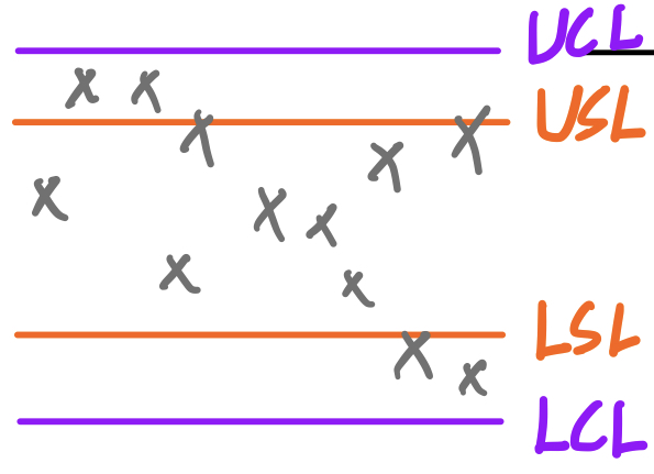
Specification & Control limits

• 용어 정의

  • Specifications (Tolerance)

    engineering design을 고려해 정한(관측된이 아니다) 품질 허용 범위

    Ex) Specification of acceptable item USL = Upper Specification Limits LSL = Lower Specification Limits

  • Control Limits

    생산된 샘플을 보고 도출해 낸 Statistical limits으로 관측의 결과가 된다.

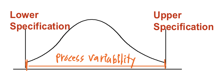
  • Process Variability

    Control Limits에 직접적으로 영향을 받으며 Specification과 독립이다.

    Process Variability = UCL - LCL

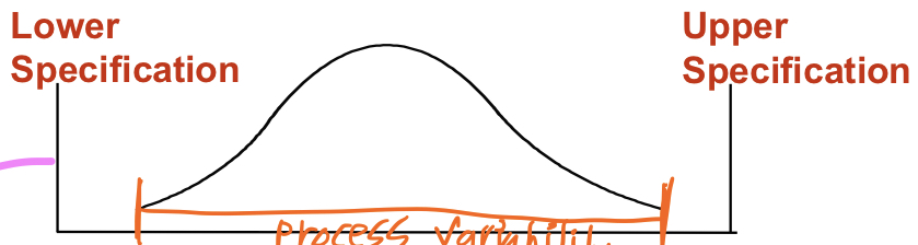
• Specification 과 Control Limits(Process variability) 의 세 가지 관계

  • A. Process variability matches Specifications

    

  • B. Process Variability well within specifications

    

    

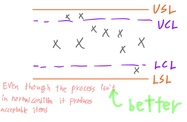
  • C. Process Variability exceds specifications

    

    

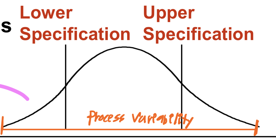
    → Even though the process is in control it produce defective units

Process Capability

• Process와 Specification의 mean이 동일할 때 Process Centered 상태라고 한다.

  이 때 Process capability ratio 를 $C_p$로 표기한다.

  $C_p = \frac{\mathrm{Specification\ width}}{\mathrm{process\ width}} = \frac{\mathrm{Upper\ specification - Lower\ specification}}{6\sigma}$

• 둘의 mean이 일치하지 않을 땐 $C_{pk}$를 사용한다.

  $C_{pk}=\min\left({\frac{\bar{\mathrm{x}}-\mathrm{LSL}}{3\sigma},\ \frac{\mathrm{USL}-\bar{\mathrm{x}}}{3\sigma}}\right)$

  $\bar{\mathrm{x}}$는 프로세스의 Mean이다.

• $C_p$ 또는 $C_{pk}$가 1보다 크다면 프로세스는 Capable 하다고 판단한다. (세가지 관계 중 A, B에 속함) 작다면, Incapable하다고 판단할 수 있다. (세가지 관계 중 C에 속함)
• Control limits와 Specification Limits를 혼동하지 말것
  • 프로세스는 Control 상태일지라도 (spec에)Incapable 할 수 있으며
  • out of Control이더라도 Capable할 수 있다.

Forecasting

개요

• Forecasting 이란?
  • A statement about the { future value of a { variable of interest } }
  • A tool used for predicting { future demand based on { past demand information } }
  • 여기선 수요 예측이라 할 수 있다. predict of demand
• Forecasting 의 효용
  • Strategic planning ( long range planning )
  • Finance and accounting ( budgets and cost controls )
  • Marketing ( future sales, new products )
  • Production and operations
• Forecasts의 features
  • 과거 사건의 데이터로 미래를 예측하는것
  • randomness 요소가 많아 정확한 예측은 불가능
  • 한가지 특정 요소에 대한 예측보단 그룹에 대한 예측이 더 정확하다.
  • 현재로부터 시간이 멀어질 수록 예측의 정확성은 감소한다.

Steps in Forecasting Process

1. Determine purpose of forecast
2. Establish a time horizon
3. Select a forecasting technique
4. Obtain, clean and analyze data
5. Make the forecast
6. Monitor the forecast

Types of Forecasts

• Judgemental: uses subjective inputs
  • 주관적 정보를 이용한 예측 (Ex. consumer surveys)
• Time series: uses historical data, assuming the future will be like the past
  • 과거 사건을 기반으로 미래를 예측
• Associative models: uses explanatory variables to predict the future
  • 대상과 연관된 변수들을 조합하여 미래를 예측

Types of Forecasts

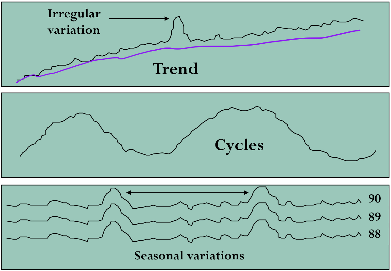
• Time Series Forecast 상세

• Trend: long-term movement in data
• Cycles: wavelike variations of more than one year’s duration
  • 총선시기, 대선시기, 올림픽시즌
• Seasonality: short-term regular variations in data
  • Calendar or time of day
    • 음식점의 점심시간 수요, 저녁 시간 수요 의 주기성
• Irregular variations: caused by unusual circumstances
  • 파업, 기상 변동
• Random variations: caused by chance
  • COVID-19

Naive Forecasts

• forecast for any period equals the previous period’s actual value
  • 당기의 전망은 전기의 관측 데이터와 정확히 일치할 것이다라는 예측
• Notations & Relations
  • Notation
    • $F(t)$ : Forecast for time t
    • $A(t)$: Actual value of a variable at time t
  • Relations

    • Stable time series data 가정

      $F(t) = A(t-1)$

    • Seasonal variations 상황 가정

      $F(t) = A(t-n)$ (n은 season 주기)

    • Data with trends 상황 가정

      $F(t)=A(t-1)+(\ A(t-1)-A(t-2)\ )$

      (일정한 기울기)

Techniques for Averaging

• Notations
  • Moving average
    • $\mathrm{F_t}$ : Forecast for time period t
    • $\mathrm{MA_n}$ : n period moving average
    • $\mathrm{A_{t-1}}$ : Actual in period t-1
    • $\mathrm{n}$ : Number of periods (data points) in the moving average
  • Weighted Moving Averages
    • $\mathrm{WMA_n}$ : n period weighted moving average
    • $\mathrm{W_i}$ : Weight $(\mathrm{W_1+W_2+…+W_n=1})$
  • Exponential Smooting
    • $\alpha$: Smoothng Constant
• Moving average

  • Recent Actual values들을 이용해 평균을 내는 방법, 새로운 Actual value가 추가될 때 마다 업데이트를 해주어야 한다.

    $\mathrm{F_t = MA_n=\frac{A_{t-n}+…+A_{t-2}+A_{t-1}}{n}}$ (최근 n년간의 Moving average)

• Weighted moving average

  • 최신의 관측치 일수록 더 높은 가중치를 주어 최신의 데이터의 영향력 제고

    $\mathrm{F_t = WMA_n=W_nA_{t-n}+…+W_2A_{t-2}+W_1A_{t-1}}$

• Exponential smoothing

  • 각 기의 예측들은 전기의 예측치에 전기 예측 오차의 $\alpha$배 만큼을 더하여 산정한다.

    Next forecast = previous forecast + $\alpha$(Actual - prev forecast)

    $\mathrm{F_t=F_{t-1}+}\alpha(\mathrm{A_{t-1}-F_{t-1}})$

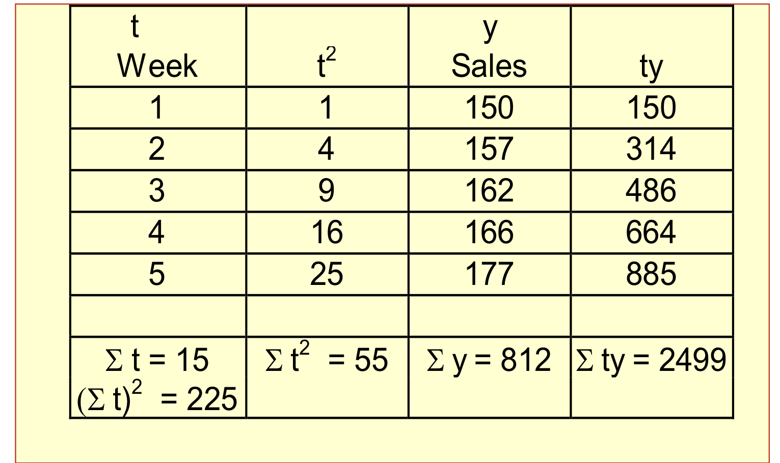
Linear Trend Equation

• Notation
  • $\mathrm{F_t}$ : Forecast for period t
  • $\mathrm{t}$ : Specified number of time periods
  • $\mathrm{a}$ : Value of $\mathrm{F_t}$ at $\mathrm{t=0}$
  • $\mathrm{b}$ : Slope of the line
• $\mathrm{F_t=a+bt}$
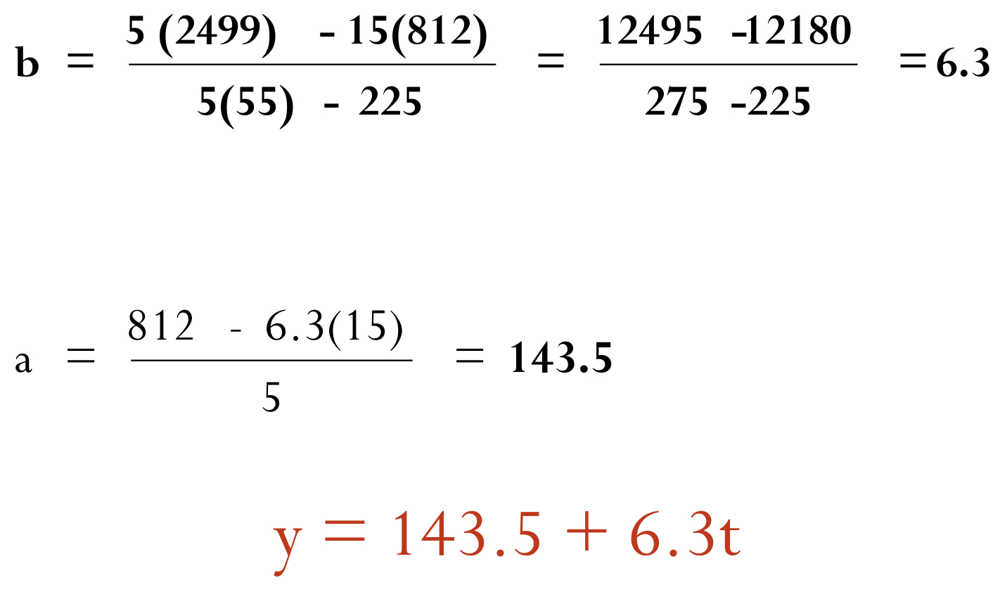
• $\mathrm{b=\frac{n\Sigma(ty)-\Sigma t\Sigma y}{n\Sigma t^2 - (\Sigma t)^2}}$
• $\mathrm{a = \frac{\Sigma y - b\Sigma t}{n}}$

• 예제

  y와 t가 문제에서 주어지면 Linear Trend Equation을 산출하는게 문제

  

  

Forecast Accuracy (MAD, MSE)

• 용어 정리
  • Error: difference between actual value and predicted value

  • Mean Absolute Deviation (MAD)

    Average absolute error $ $ $\mathrm{MAD=\frac{\Sigma\ |\ Actual-forecast\ |\ }{n}}$

    • Weights errors linearly

  • Mean Squared Error (MSE)

    Average of squared error

    $\mathrm{MSE=\frac{\Sigma\ (Actual-forecast)^2\ }{n}}$

    • More weight to large errors

Scheduling

개요

• Scheduling 이란?
  • Establishing the timing of the use of equipment, facilities, and human activities
• Scheduling의 효용
  • Cost savings
  • Increases in productivity
  • reduces Throughput Losses
• 두가지 중점 사안

  • Loading

    일을 어디에 배치하는가

  • Sequencing

    어떤 순서로 일을 처리하는가 -priority rules

Loading

• 투입요소와 산출요소
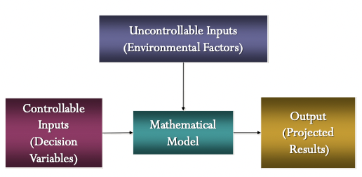
  • Inputs
    • Controllable Inputs ( Decision Variables )
    • Uncontrollable Inputs ( Environmental Factors )
  • output ( Project Results)
  • Mathematical Model
    • Inputs 를 Outputs로 변환하는 수학식

  • 개략도

    

• Linear Programming(LP) Problem
  • objective
    • 해 들을 평가하는 기준으로 해가 갖는 어떤 특성이 최대한 충족해야할 조건에 대한 표현
  • feasible solution
    • 모든 제약들을 만족하는 해
  • optimal solution
    • feasible solution 중 objective를 충족하는 최적의 해
• LP 조건하 Loading Formulation
  • Notation
    • $\mathrm{x_{ij}}=\begin{cases}1&\mathrm{if\ agent\ i\ is\ assigned\ to\ task\ j} \ 0 &\mathrm{otherwise}\end{cases}$
    • $\mathrm{c_{ij}}=\mathrm{cost\ of\ assigning\ agent\ i\ to\ task\ j}$

  • Formulation

    $\mathrm{Min\ \Sigma_i(\Sigma_jc_{ij}x_{ij})}$

    $\mathrm{s.t.\ \ \Sigma_jx_{ij}=1\ \ for\ each\ agent\ i}$

    $\mathrm{\ \ \ \ \ \ \ \Sigma_ix_{ij}=1\ \ for\ each\ agent\ j}$

    $\mathrm{\ \ \ \ \ \ \ x_{ij}=0\ or\ 1\ \ for\ all\ i\ and\ j}$

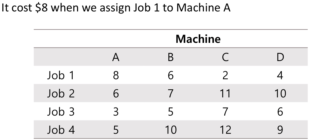
  • 예제

    

    Formulation

    Min{$\mathrm{8x_{A1}+6x_{B1}+2x_{C1}+4x_{D1}}$

    $\mathrm{+6x_{A2}+7x_{B2}+11x_{C2}+10x_{D2}}$

    $\mathrm{+3x_{A3}+5x_{B3}+7x_{C3}+6x_{D3}}$

    $\mathrm{+5x_{A4}+10x_{B4}+21x_{C4}+9x_{D4}}$}

Sequencing

• 개요
  • Priority rules
    • Simple heuristics used to select the order in which jobs will be processed
  • Job Time
    • Time needed for setup and processing of a job
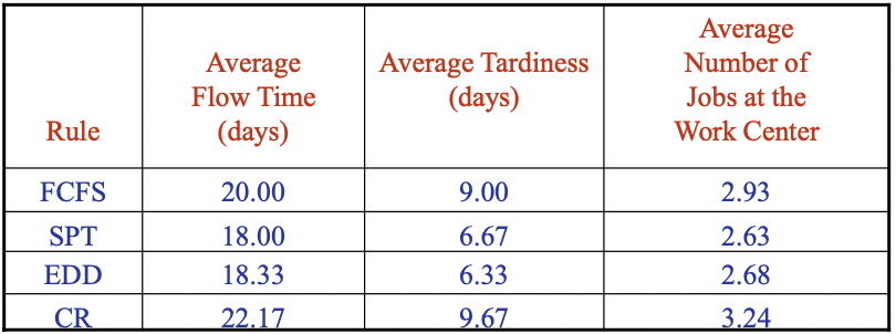
• Priority Rules
  • 종류
    • FCFS: First Come First Served
    • SPT: shortest processing time
    • EDD: earliest due date
    • CR: Critical ratio
      • Critical = (remaining time) / (process time)
      • remaining time can be minus
    • Rush: emergency or preferred customers first
  • 측정기준
    • Job flow time
      • 하나의 작업(일)이 처리되기까지 소요시간
      • 대기시간을 포함한다.
    • Job lateness
      • lateness = (Completion time) - (due date)
      • tardiness = lateness (if lateness < 0 → tardiness = 0)
    • Makespan
      • 모든 일을 처리하기까지 소요되는 시간
      • 첫 job의 processing이 시작될 때부터 마지막 job이 끝날 때까지 시간간격
    • Average number of jobs
      • Total flow time / Makespan
      • makespan의 기간에 처리되지 않은 작업의 평균 개수
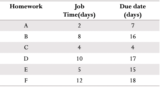
  • 예제

    • problem

      

    • SOL

      

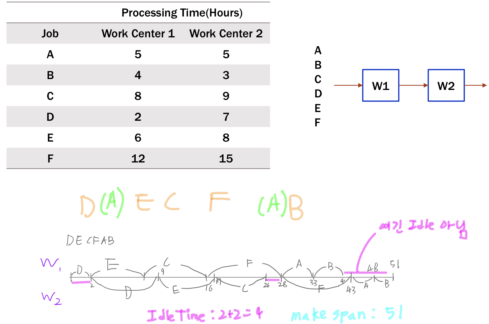
Johnson’s Rule

• 사용 조건
  • 모든 작업 시간은 각각 독립이고, 확정적이어야 한다.
  • 선행작업이나 후행작업 등의 관계가 설정되어 있지 않아야 한다.
  • 작업은 모두 2개의 work center를 거쳐 완제품이 되어야 한다.
  • 각 작업이 거치는 work center의 순서는 동일해야 한다.
• Johnson’s Rule Optimum Sequence
  1. 모든 작업을 Work Center의 종류에 관계 없이 둘중 작은 processing time을 산출한다.
  2. 산출한 결과를 바탕으로 정렬한다.
  3. 정렬된 job list에서 작은 processing time을 갖는 job을 꺼낸다.
  4. job 의 processing time이 속한 Work Center에 따라 다음을 진행한다. a. WC1일 경우 sequence list 앞에서부터 쌓아 올린다. b. WC2일 경우 sequence list 뒤에서부터 쌓아올린다.
  5. job list가 empty일 때까지 3, 4를 진행한다.

• 예제

  

Aggregate Planning

개요

• Aggregate Planning 이란?

  • 중기적인 capacity planning (2 ~ 12개월 앞의 미래를 뜻한다.)

    

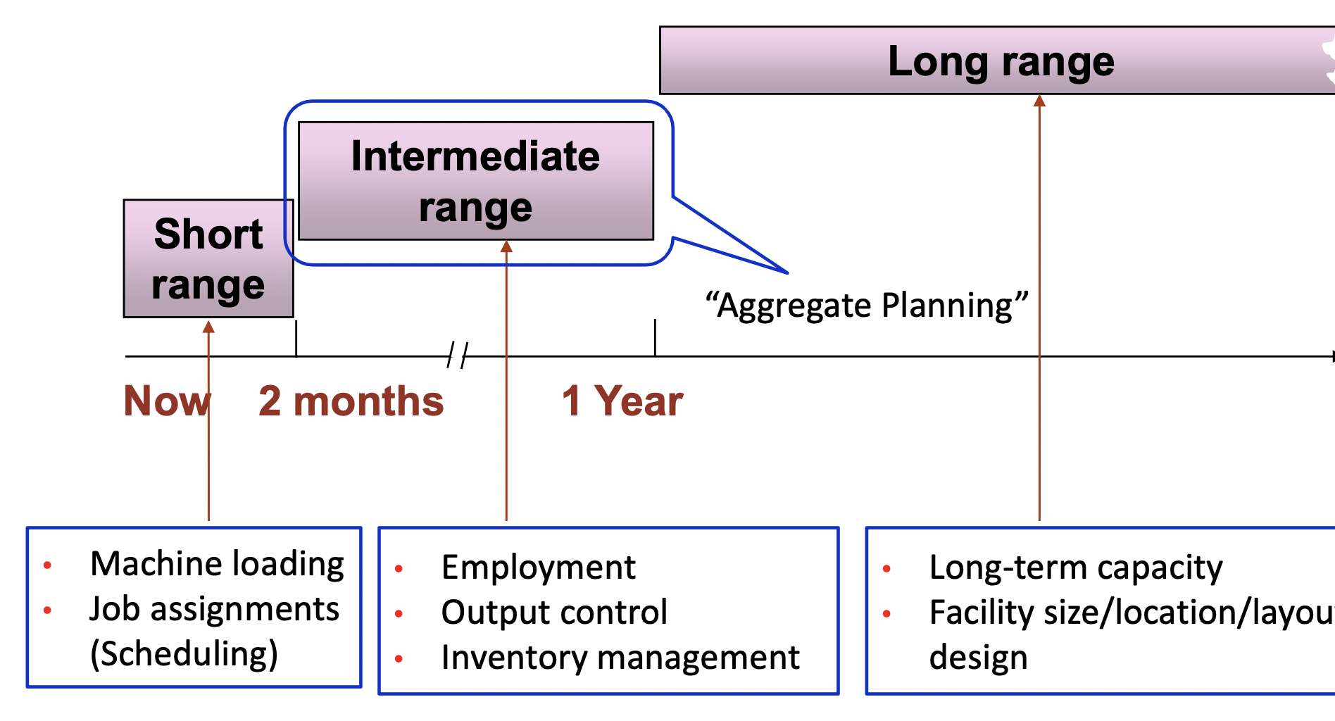
  • 특정 모델의 생산에 대한 계획을 짜는 것이 아니라 어떤 제품군의 생산을 계획하는 것

    

    Ex. 현대 모터스: 아반떼 100대, 소나타 100대, … → X 승용차 1000대, 트럭 200대,…. → O

• 조정 요소
  • Proactive : alter demand to match capacity (능동적으로 demand 조정)

    • Pricing

      Ex. 조조할인을 통한 수요 분산

    • Promotion

      Ex. 블랙프라이데이 세일을 이용한 비선호품 수요 증가 재고처리,

    • Back orders

      수요가 감당 못하게 많을 때 대기열을 생성하여 수요 소폭 하향, 납품 기한 연장

    • New demand

      신체품 출시로 새로운 수요를 창조

  • Reactive: alter capacity to match demand ← 이것에 초점을 두고 본다.
    • Hire and lay off worker (고용, 해고)
    • Overtime / slack time (초과근무, 납품지연)
    • Part-time workers (아르바이트)
    • Inventories (재고 관리)
    • Subcontracting (하청)
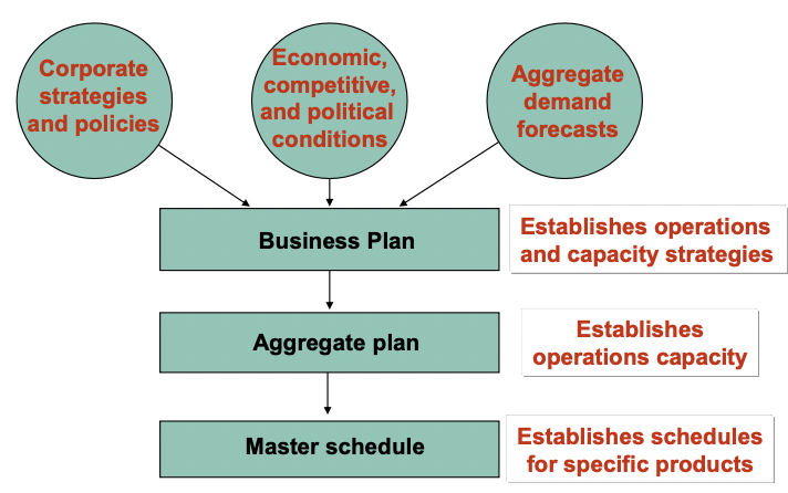
• Production plan은 aggregate planning의 결과물이다.
• Plan을 주기적으로 업데이트 해주어야 한다.
  • 12 - 18개월 앞을 항상 내다 볼 수 있도록 최신화 시켜주어야 한다.

Aggregate Planning Inputs

• Resources
  • Workforce
  • Facilities
• Costs
  • Inventory carrying
  • Back orders
  • Hiring/Fireing
  • Overtime
  • Inventory changes
  • Subcontracting
• Demand forecast
• Policies
  • Subcontracting (how much /N)
  • Overtime (how much /N)
  • Inventory levels (how much / N)
  • Back orders (how much /N)

Aggregate Planning outputs

• Total Cost of a plan
• Projected levels of
  • Inventory
  • output
  • Employment
  • Subcontracting
  • Backordering

Basic Strategies

• 상황 제시

  

• 사용 전략

  • Level capacity strategy

    

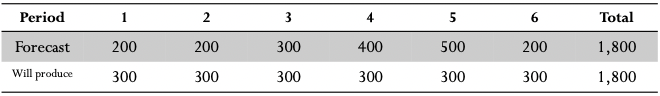
    • 정상 작업시간 내의 생산역량을 일정하게 유지하는 전략
    • 실 수요에 따라서 policies에 입각해 대처
    • 장점 안정적인 생산역량 유지
    • 단점 재고 비용이 증가할 수 있음 초과근무비용, idle time 이 증가할 수 있다. utilization이 낮아질 수 있다.

  • Chase demand strategy

    • 수요에 맞게 생산역량(capacity)을 그때그때 조정
    • Forecast와 planned output은 세트로 움직인다.
    • 장점 재고비용 감소 utilization 이 높게 유지됨(+보통 고용보단, overtime을 사용)
    • 단점 생산량 또는 노동력을 조정하는데 드는 비용이 높다.

Relations

• Number of workers in a period = Num of workers at end of prev period + Number of new workers at start of period - Number of laid-off workers at start of the period
• Inventory at the end of a period = Inventory at the end of the previous period + production in the current period - Amount used to satisfy demand in the current period
• Average inventory = $\mathrm{\frac{Beginning\ inventory+Ending\ inventory}{2}}$
• Cost for a period = Output cost + Hire/lay-off cost + Inventory cost + Back-order cost *Output cost = Regular work cost + Overtime cost + Subcontract cost

Material requirements planning (MRP)

개요

• 최종 생산물을 만들기 위해 여러 반제품들이 필요한 생산 공정의 Planning

• 개략도

  

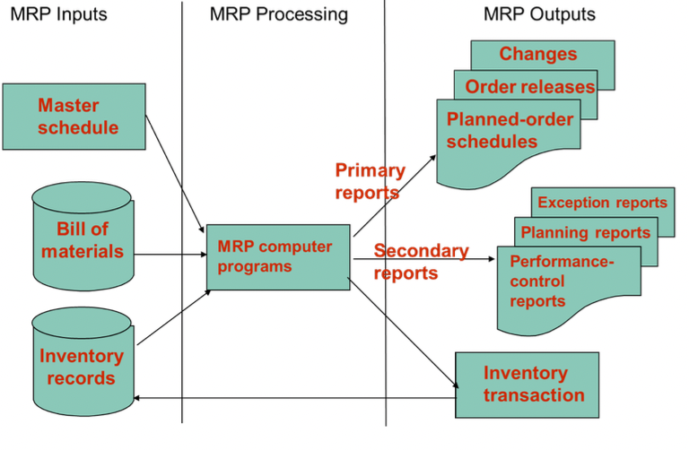
Inputs

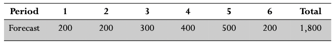
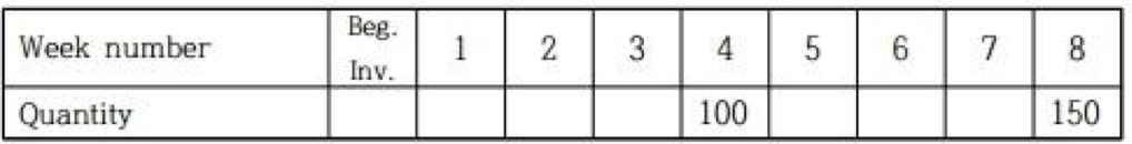
• Master Schedule
  • 어떤 제품/반제품이 언제까지 얼마나 생산되어야 하는지에 대한 문서

  • 예시

    

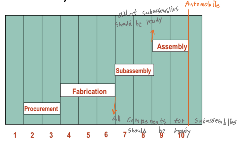
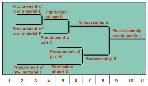
  • cumulative lead time

    모든 요소들의 lead time (조달기한) 의 누적

• Bill of materials (BOM)
  • 최종 생산물의 완성에 필요한 모든 원제료, 부속 그리고 조립 공정까지에 대해 적힌 명세서
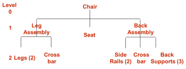
  • Product structure tree

    • BOM을 tree 형태로 시각화 한 것

      

• Inventory Records
  • 다음의 item에 대해 기한과 함께 명시해 놓은것
    • Gross requirements
    • Scheduled receipts
    • Amount on hand
    • Lead times
    • Lot size
    • etc…
  • Net requirements = Gross req - available Inventory
  • Available Inventory = Projected on hand - Safety stock - Inventory allocated to other items *이 단원 내에서 safety stock과 inventory allocated to othre items 는 0으로 가정

  • 예시

    

개념 간단 정리

• Gross requirements
  • Total expected demand for an item during each time period without regard to the amount on hand
  • 내가 지금 몇개 가지고 있는지와 관계 없이 해당 기간 내에 필요한 item의 수량
  • 어떤 생산물 A을 생산하기 위한 부속 b의 경우 A의 planned-order releases에서 정보를 얻을 수 있다.
• Scheduled receipts
  • Open orders scheduled to arrive from vendors or elsewhere by the beginning of a period
  • 해당 기간 시작일에 예약으로 들어온 item 수량
• Planned on hand
  • 어떤 기간의 시작일에 내가 보유하고 있을 것으로 예상되는 item 수량
  • = 전기의 Scheduled receipts + 전기의 available inventory
• Net requirements
  • Gross - inventory we have
• Planned-order receipts
  • Quantity expected to received at the beginning of the period
  • 해당 기간 초까지 생산 완료 되어야 할 수량
• Planned-order releases
  • 해당 기간에 초까지 생산 준비 되어야 할 수량 (준비되어야 할 반제품들의 세트)
    • Planned-order releases = Planned-order receipts / (1-불량률) 불량률은 아직 고려 안하니 둘을 같다고 보면된다.

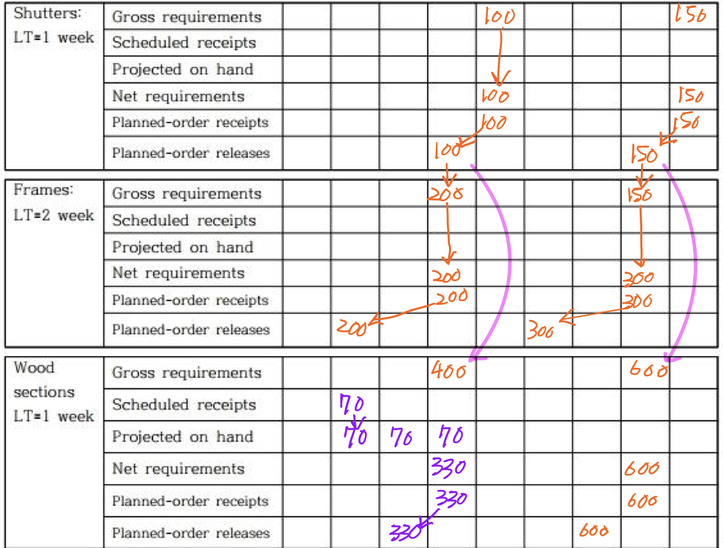
table 예시

• Master schedule

  

• Shutter = Frame(2) + Wood section(4)

• Table